Background
This section is intended to give some insights into the mathematical background that is the basis of PyTrajectory.
Contents
Trajectory planning with BVP’s
The task in the field of trajectory planning PyTrajectory is intended to perform, is the transition of a control system between desired states. A possible way to solve such a problem is to treat it as a two-point boundary value problem with free parameters. This approach is based on the work of K. Graichen and M. Zeitz (e.g. see [Graichen05]) and was picked up by O. Schnabel ([Schnabel13]) in the project thesis from which PyTrajectory emerged. An impressive application of this method is the swingup of the triple pendulum, see [TU-Wien-video] and [Glueck13].
Collocation Method
Given a system of autonomous differential equations
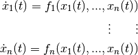
with ![t \in [a, b]](../_images/math/7ee1e80a90cec6b0dea8088399ebb8442e81fc28.png) and Dirichlet boundary conditions
and Dirichlet boundary conditions

the collocation method to solve the problem basically works as follows.
We choose  collocation points
 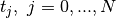 from the interval
![[a, b]](../_images/math/1d2d3c2141e9f7387a2d26b1ea40c2aabd96f3ac.png) where
where 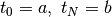 and search for functions
![S_i:[a,b] \rightarrow \mathbb{R}](../_images/math/9cf43e534d51d3477a6567b4cd77eee244f39c2c.png) which for all
which for all  satisfy the
following conditions:
satisfy the
following conditions:
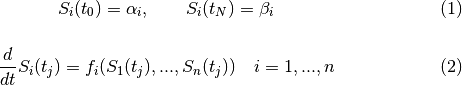
Through these demands the exact solution of the differential equation system will be approximated.
The demands on the boundary values  can be sure already by suitable
construction of the candidate functions. This results in the following system of equations.
can be sure already by suitable
construction of the candidate functions. This results in the following system of equations.
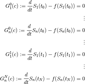
Solving the boundary value problem is thus reduced to the finding of a zero point
of 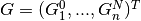 , where
  is the vector of all independent
parameters that result from the candidate functions.
is the vector of all independent
parameters that result from the candidate functions.
Candidate Functions
PyTrajectory uses cubic spline functions as candidates for the approximation of the
solution. Splines are piecewise polynomials with a global differentiability.
The connection points  between the polynomial sections are equidistantly
and are referred to as nodes.
between the polynomial sections are equidistantly
and are referred to as nodes.
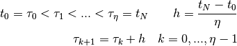
The  polynomial sections can be created as follows.
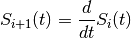
Then, each spline function is defined by
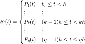
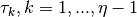
The spline functions should be twice continuously differentiable in
the nodes  . Therefore, three smoothness conditions can be set up in all
 .
.
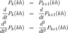
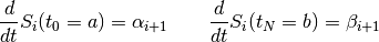
In the later equation system these demands result in the block diagonal part of the matrix. Furthermore, conditions can be set up at the edges arising from the boundary conditions of the differential equation system.
The degree  of the boundary conditions depends on the structure of the differential
equation system. With these conditions and those above one obtains the following equation system
(
of the boundary conditions depends on the structure of the differential
equation system. With these conditions and those above one obtains the following equation system
( ).
).
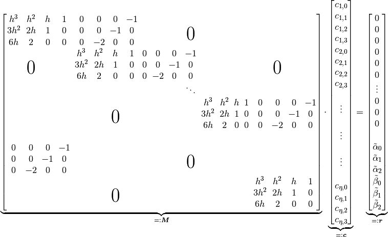
The matrix  of dimension
 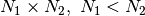 , where
  and
and  , can be decomposed
into two subsystems
, can be decomposed
into two subsystems 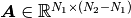 and
and  .
The vectors
.
The vectors  and
and  belong to the two matrices with the respective coefficients of
  .
.
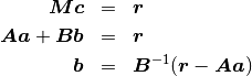
With this allocation, the system of equations can be solved for and the parameters in
remain as the free parameters of the spline function.
Note
Optionally, there is available an alternative approach for defining the candidate functions, see Non-Standard Approach.
Use of the system structure
In physical models often occur differential equations of the form

For these equations, it is not necessary to determine a solution through collocation. Without severe impairment of the solution method,
it is sufficient to define a candidate function for  and to win that of
  by differentiation.
Then in addition to the boundary conditions of  applies
Similar simplifications can be made if relations of the form  arise.
Levenberg-Marquardt Method
The Levenberg-Marquardt method can be used to solve nonlinear least squares problems. It is an extension of the Gauss-Newton method and solves the following minimization problem.

The real number  is a parameter that is used for the attenuation of the step size
  and is free to choose.
Thus, the generation of excessive correction is prevented, as is often the case with the Gauss-Newton method and leads to a possible
non-achievement of the local minimum. With a vanishing attenuation,
and is free to choose.
Thus, the generation of excessive correction is prevented, as is often the case with the Gauss-Newton method and leads to a possible
non-achievement of the local minimum. With a vanishing attenuation,  the Gauss-Newton method represents a special case
of the Levenberg-Marquardt method. The iteration can be specified in the following form.
the Gauss-Newton method represents a special case
of the Levenberg-Marquardt method. The iteration can be specified in the following form.

The convergence can now be influenced by means of the parameter . Disadvantage is that in order to ensure the convergence,
must be chosen large enough, at the same time, this also leads however to a very small correction. Thus, the Levenberg-Marquardt
method has a lower order of convergence than the Gauss-Newton method but approaches the desired solution at each step.
Control of the parameter 
The feature after which the parameter is chosen, is the change of the actual residual
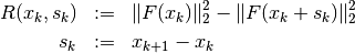
and the change of the residual of the linearized approximation.

As a control criterion, the following quotient is introduced.
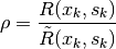
It follows that  and for a meaningful correction
  must also hold.
Thus,
must also hold.
Thus,  is also positive and
  for
for  .
Therefor should lie between 0 and 1. To control two new limits
.
Therefor should lie between 0 and 1. To control two new limits  and
and  are introduced
with
are introduced
with  and for
  we use the following criteria.
 is doubled and
  is recalculated
 in the next step is maintained and is used
 is accepted and is halved during the next iteration
Handling constraints
In practical situations it is often desired or necessary that the system state variables comply with certain limits. To achieve this PyTrajectory uses an approach similar to the one presented by K. Graichen and M. Zeitz in [Graichen06].
The basic idea is to transform the dynamical system into a new one that satisfies the constraints. This is done by projecting the constrained state variables on new unconstrained coordinates using socalled saturation functions.
Suppose the state  should be bounded by
  such that
  for all
 ![t \in [a,b]](../_images/math/31bd8867031ba0d2c1137e9a2c9832cfe472d99b.png) .
To do so the following saturation function is introduced
.
To do so the following saturation function is introduced

that depends on the new unbounded variable  and satisfies the saturation limits
  , i.e.
 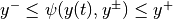 for all
  . It is assumed that the limits
are asymptotically and
. It is assumed that the limits
are asymptotically and  is strictly increasing , that is
  .
For the constraints
.
For the constraints ![x \in [x_0,x_1]](../_images/math/1063c2328a7654f2dd6219947f98440d9e3da666.png) to hold it is obvious that
to hold it is obvious that  and
and  . Thus the constrained
variable is projected on the new unconstrained varialbe .
. Thus the constrained
variable is projected on the new unconstrained varialbe .
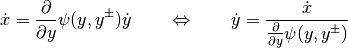
By differentiating the equation above one can replace  in the vectorfield with a new term for
  .
.
Next, one has to calculate new boundary values  and
and  for the variable from those,
 and
and  , of .
This is simply done by
, of .
This is simply done by

Now, the transformed dynamical system can be solved where all state variables are unconstrained. At the end a solution for the original state
variable is obtained via a composition of the calculated solution  and the saturation function .
There are some aspects to take into consideration when dealing with constraints:
- The boundary values of a constrained variable have to be strictly within the saturation limits
- It is not possible to make use of an integrator chain that contains a constrained variable
Choice of the saturation functions
As mentioned before the saturation functions should be continuously differentiable and strictly increasing. A possible approach for such functions is the following.
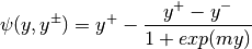
The parameter  affects the slope of the function at
  and is chosen such that
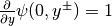 , i.e.
An example
For examples on how to handle constraints with PyTrajectory please have a look at the Examples section, e.g. the Constrained double integrator or the Constrained swing up of the inverted pundulum.
References
| [Graichen05] | Graichen, K. and Hagenmeyer, V. and Zeitz, M. “A new approach to inversion-based feedforward control design for nonlinear systems” Automatica, Volume 41, Issue 12, Pages 2033-2041, 2005 |
| [Graichen06] | Graichen, K. and Zeitz, M. “Inversionsbasierter Vorsteuerungsentwurf mit Ein- und Ausgangsbeschränkungen (Inversion-Based Feedforward Control Design under Input and Output Constraints)” at - Automatisierungstechnik, 54.4, Pages 187-199, 2006 |
| [Graichen07] | Graichen, K. and Treuer, M and Zeitz, M. “Swing-up of the double pendulum on a cart by feed forward and feedback control with experimental validation” Automatica, Volume 43, Issue 1, Pages 63-71, 2007 |
| [Schnabel13] | Schnabel, O. “Untersuchungen zur Trajektorienplanung durch Lösung eines Randwertproblems” Technische Universität Dresden, Institut für Regelungs- und Steuerungstheorie, 2013 |
| [TU-Wien-video] | Glück, T. et. al. “Triple Pendulum on a Cart”, (laboratory video), https://www.youtube.com/watch?v=cyN-CRNrb3E |
| [Glueck13] | Glück, T. and Eder, A. and Kugi, A. “Swing-up control of a triple pendulum on a cart with experimental validation”, Automatica (2013), doi:10.1016/j.automatica.2012.12.006 |